14.                                      
   Modeling of System Performance

The primary reason for creating a computer model of a solar energy system is to determine how much solar-derived energy the system will supply over a long period of time.  As with any analytical model, the characteristics of the components and their sizes may be varied to help the engineer optimize the design of a system in terms of system performance and cost.  Figure 14.1 shows some of the more important inputs and outputs for a typical analytical model of an industrial solar energy system.

 

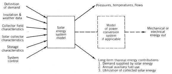
Figure 14.1  Block diagram of a typical analytical model of a solar energy system

Long-term system performance is important in determining the economic viability of a particular system design.  Using a computer model of a particular system and time-dependent weather data for a particular site, the designer can determine how much solar derived energy can be delivered to a specific energy demand.  This is typically done by performing hour-by-hour energy balances over a "typical" year's insolation and ambient-temperature data.

14.1  Underlying Assumptions

 

Although analytically much easier to use, average yearly or even average monthly insolation data can grossly misrepresent long-term system performance when the collector subsystem interfaces with other subsystems such as energy storage. Significantly different amounts of energy collected and utilized would be predicted, for example, for a solar energy system operating for a month with long periods of clear days and long periods of cloudy days, than for a month in which every day was the same and had insolation equal to the average monthly insolation. As a part of the design of a solar system, therefore, it is considered best to develop a computer model of that system and use it to evaluate the yearly performance of the system using "typical" hour-by-hour weather data for the specific site where it is to be located.

 

The underlying principle of most computer-based system models is the concept of energy accounting using the first law of thermodynamics.  Since the amount of solar energy entering a system varies, the typical computer model performs a steady-state energy balance over a short period of time (usually one hour) and then sums these energies to provide what appears over the long term to be a continuous description of the energy flows into and out of the system.

 

In this chapter we develop a simple computer design model that has many of the characteristics of the larger computer models used for detailed design optimization of commercial systems.  The accuracy of the system model may be enhanced by using some of the detailed algorithms developed in subsequent chapters.

 

The basic philosophy used here in developing a computer design tool to aid the system designer is to construct a simple energy accounting and system control algorithms that can accept input that can range from very simple to very complex.  This is illustrated in Figure 14.2.  The energy accounting and system control part of this program is called SIMPLESYS.  A simplified stand-alone version of SIMPLESYS will be developed later in this chapter.

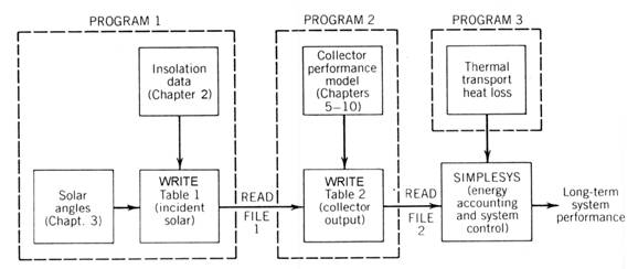
Figure 14.2  Example of the building block approach to computer modeling of a solar energy system.

The basic energy accounting code acts only as a manipulator of energy data as defined by the system requirements.  The building block approach allows the designer to build up a system model of almost any degree of sophistication without any one piece becoming unwieldy.

 

PROGRAM 1 computes the solar angles developed in Chapter 3, applies these to a solar irradiation data file and generates FILE 1 which is a table of hourly values of the local solar irradiation incident on the collector aperture.

 

PROGRAM 2, in turn, is then run using FILE 1 along with a solar collector performance model to compute the collector output.  The model for solar collector performance can vary anywhere from actual test data to a complete thermo/optical description of the collector.  Simplified collector performance models are described in Chapter 5 through Chapter 9.  PROGRAM 2 then produces TABLE 2, a table of hour-by-hour collector field output, which is then read into SIMPLESYS.  Likewise, PROGRAM 3 could contain a number of calculations that would accurately predict the thermal losses in the thermal transport systems.

 

Energy losses from the collector field calculated in PROGRAM 3 along with the collector field output from PROGRAM 2 provide the energy inputs into SIMPLESYS.  These in turn, along with stored and auxiliary energy sources, provide for the energy balance and control function choices of SIMPLESYS and the prediction of long-term solar energy system performance.

 

This chapter describes the structure of SIMPLESYS and then illustrates its use using highly simplified inputs for PROGRAMS 1, 2 and 3.  By the end of this chapter, the reader should have an understanding of how this model works, and the effects on system design of varying the size of the collector field, of the thermal energy storage, heat loss and demand.  These interactions encompass the major considerations in solar energy system design as is discussed in detail in Chapter 15.

14.2  A Simple Solar Energy System Model - SIMPLESYS

At this point we will start to develop a complete but simplified, stand-alone solar energy system model based on the system shown schematically in Figure 14.3.  A list of the program variables noted on this figure is given in Table 14.1.

 

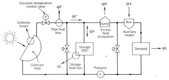
Figure 14.3  Schematic diagram of a simple solar energy system.

Table 14.1  Computer Variables Used in Program SIMPLESYS

From auxiliary                                          QA                            EA                        YA

From collector field                                  QC                            EC                        YC

To dissipation device                               QD                            ED                        YD

To demand                                              QL                             EL                        YL

Added to storage (+ is in, - is out)           QS                          ZS,ES                     YS

Storage Loss                                           SL                                                          

Other Variables

CM                   maximum (noon) rate of energy flow from collector field (kW)

D                      day number

EP                    energy to heat piping to operating temperature (kWh)

ES                    energy in storage at any given time (kWh)

M                      system operating mode number

OFF                 time system is turned off (h)

QF                   rate of heat loss from field piping (kW)

RT                    hour angle from noon (radians)

SL                    rate of heat loss from storage (KW)

SM                   maximum amount of energy which can be stored (kWh)

START             time system is started (h)

SU                    sum of energy required to "start up" collector field (kWh)

T                      time (24 hour clock) (h)

ZS                    net energy into storage for the day (kWh)

 

For the maximum understanding of how a solar energy system works and the techniques and assumptions required for analytical modeling of that system, it is suggested that the reader try changing the values of different input parameters and see what happens to the other system variables.

 

Program SIMPLESYS is included on this web site as a separate tab on the home page and all of the initial pages of the site.  We have also included a link below.

 

Run Program SIMPLESYS

 

14.2.1       System Description and Control Logic

Probably the best place to start modeling a solar energy system is by defining how the system is to be operated and what the operating priorities are.  The typical system configuration shown in Figure 14.3 will provide thermal energy to a demand either directly from the solar collector field at the rate QC, from the storage at the rate (-)QS, or from an auxiliary heater (typically fired by natural gas or oil) at the rate QA.  A means of dissipating excess energy at the rate QD is provided, usually in the form of a forced-draft heat exchanger or a cooling tower and/or deactivating some of the solar collectors.

 

Major heat losses are represented by two terms; the rate of heat loss from the field piping QF and the rate of heat loss from the storage SL.  Many valves and pumps have been omitted from Figure 14.3 for simplicity.

 

For this system model, the rate of thermal energy going to the demand is selected from the collector field, the storage or the auxiliary heater in that order of priority. A plot of how the demand QL may be supplied on a typical day is shown in Figure 14.4. Although not necessary, the demand shown here is a constant over the full period of system operation.

 

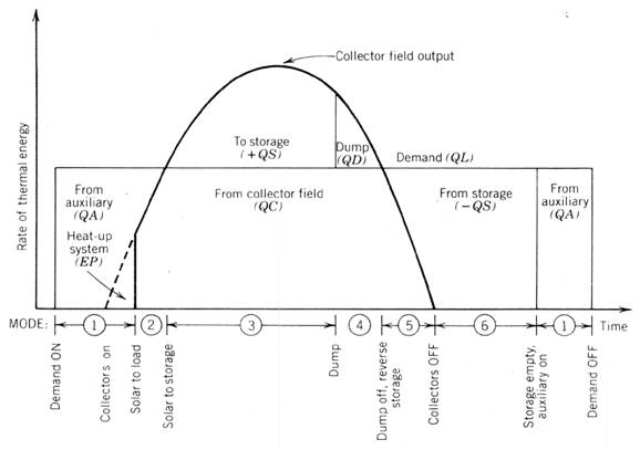
Figure 14.4  Modes of operation of a simple solar energy system with storage.

There are six possible "modes" of operation pictured in Figure 14.4 and describe s in Table 14.2. In the early morning before the sun is visible the demand is supplied completely by the auxiliary heater. This we call operation mode l. Mode 1 continues through the time when the collector field has started operation but has not yet supplied enough energy (EP)  to heat the fluid and pipe mass in the collector field to the operating temperature of the field.  Once the field piping is heated, the demand uses as much energy as is available from the collector field (QC) with the difference (QA) compensated by the auxiliary heater.  This is operation mode 2.  In operation mode 3, the rate of energy output from the collector field is greater than that required by the demand and the excess (QS) is routed into the storage.

Table 14.2.      SIMPLESYS Operating Modes

 

 

        0               System Off                           Empty                QL = 0

1               Auxiliary only                         Empty                 QA = QL

2               Auxiliary and                          Empty                 QA = QL  QC

                          collectors

3               Collectors only                      Charging            QS = QC  QL

4               Collectors only                      Full                     QD = QC  QL

5               Collectors and                       Discharging        QS = QC  QL

                           storage

This continues until the storage is full (reaches the energy level SM) and can accept no more energy.  At this point, some heat dissipation device must be operated to "dump" the excess energy (QD), which we call operation mode 4.  As the insolation decreases (i.e., in the afternoon of a clear day), the output from the collector field will again become less than that required by the demand, but this time there is stored energy (ES) to make up the difference between the collector field output and the demand.  This is noted as operation mode 5. When the collector field finally stops producing net energy, the full demand is supplied from the storage until it is fully discharged.  This is the final discrete mode of operation, which is noted here as operation mode 6.  If the system continues to operate past the time when the storage is fully discharged, mode 1 operation will begin again where the auxiliary heater supplies the full demand.

 

Energy Accounting.  The first law of thermodynamics energy flow balance for this system is

                                                            (kW)              (14.1)

where for simplicity, the heat loss rates from the collector field piping QF and the storage SL have been incorporated into the terms QC and QS, respectively.  All the energy flow terms are defined in Table 14.1.

 

     Control Logic. In this program, the control logic determines the proper mode of operation. A logic diagram showing how the different modes of operation are selected is shown in Figure 14.5. Once the mode of operation is selected, the appropriate truncated form of Equation (14.1) is solved to find QS, QD, or QA, since QL is defined and QC is determined from calculations employing sophisticated models of collector performance and local solar irradiation.  These forms of Equation (14.1) are shown in Table 14.2 for the different modes of operation. This overall operation is shown schematically in Figure 14.6 in terms of the program variables used in SIMPLESYS.

 

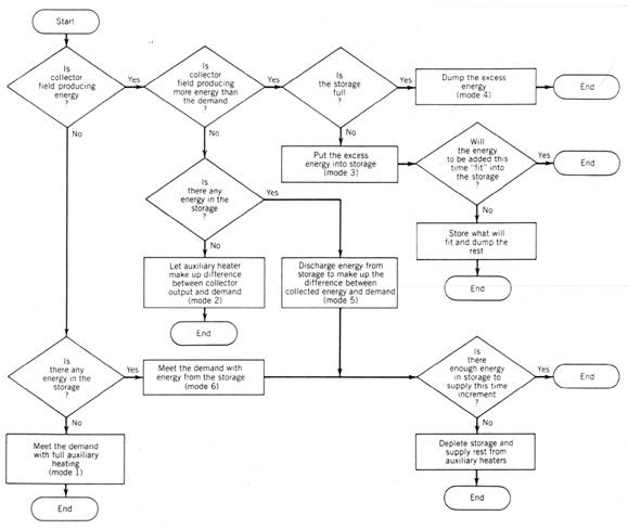
Figure 14.5  Control logic for a typical solar energy system model where the system includes storage.

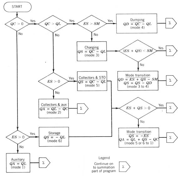
Figure 14.6  Energy flow balances for different modes of operation.

Once the energy flows have been determined for the time increment used (1-hour increments are used here, but this could be changed), the program then goes to an energy flow summation mode.  The hourly energy flows are summed over the operation day to determine the daily energy values EA, EC, ED, EL, and ZS. At the end of the day, these values are added to yearly sums YA, YC, YD, YL, and YS and then are reset to zero for the next day's totals.

 

One summation term, ES, requires particular mention.  Since stored energy may be carried over to the following day, ES is not zeroed at the end of the day. Therefore, ES represents the amount of energy accumulated in the storage at any given time.  The parameter ES differs from ZS in that ZS represents only the net amount of energy placed into or removed from storage on any particular day.

 

Figure 14.7 shows the progression of steps through program SIMPLESYS.  Two program loops are noted; the inner one occurring each hour of the day and the outer one, each day of the year.

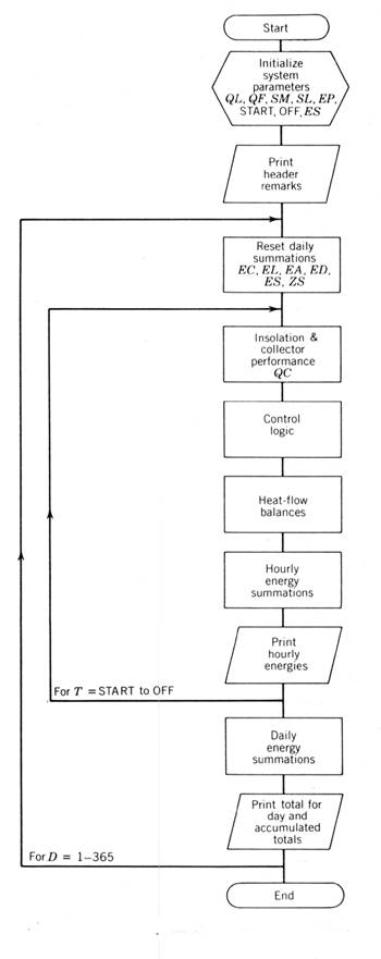
Figure 14.7  Flow diagram of program SIMPLESYS.

Collected Energy. In this section, since we want to show how a system operates rather than provide accurate solutions for specific systems, we begin with a simplistic model for giving the energy collected at any particular time.  This model gives an energy flow rate from the collector field QC that varies as a sine function with a collector field maximum output of CM (kW) at noon and zero at 6:00 AM and 6:00 PM as where T is the hour (solar time) of the day (24-hour clock where midnight is hour 0 and noon is hour 12) and the argument of the sine function in radians.  The term QF represents a constant rate of heat loss from the collector field piping.

                                                  (kW)                           (14.2)

It should be emphasized that this is a very simplistic insolation model.  In Chapter 2 we discuss what must be done to provide more realistic insolation models or recorded data.  Since the objective here is to illustrate how SIMPLESYS shows the interactions of various system components, a sinusoidal model is adequate for this purpose.

 

Collector Field Heat-up and Loss - Solar energy systems must operate for a period of time in the morning before they collect enough energy to heat the fluid, receiver, and piping in the collector field up to operating temperature.  During this initial heat-up period, the system is run in a "bypass" mode.  In SIMPLESYS, an amount of energy, specified by the user as EP (kWh) must be supplied by the collectors each morning before they can begin supplying energy to the demand.  This is done by setting up a start-up energy counter SU that, when the value EP is reached, will permit energy to pass from the collector field into the system.  A reasonable approximation of the value of EP can be found by determining the product of the mass and the specific heat of each of the materials that must be heated to operating temperature in the morning.  The overall thermal mass is then determined by adding these:

                                                             (kWh)                          (14.3)

where m_i is the mass of material i, c_p,i is its specific heat, and T_i is the temperature to which it must be heated. All of this energy is assumed to be lost overnight.

 

Since a significant amount of energy can be lost during operation from the collector field piping through its insulation, a term to account for this, QF (kilowatts) is included in the model and is subtracted directly from the energy collected by the collector field as noted in Equation (14.2).  This value may be approximated by summing the heat loss rates over all of the collector field piping in the form

                                                                (kW)                    (14.4)

where for the p ^th segment of pipe, d_o and d_i are respectively the outside and inside diameters of the insulation, L_p is the length of pipe, k_p is its thermal conductivity, and T_p is the operating temperature.

 

Storage.  The thermal energy storage in this system model could be either a thermocline type of storage medium or a latent-heat type.  All that is assumed is that when the storage is supplying energy to the system, it can supply the full amount needed by the demand QL. The storage has a capacity of SM (kilowatt-hours) of energy and loses heat to the surroundings at the rate SL (kilowatts).  This heat loss occurs as long as there is energy in the storage that can be discharged.  In a more complete model of storage, the designer may want to include cool down of the depleted storage.

 

A decision must be made initially as to how much energy is in the storage at the start of the first day's run.  This is done by giving ES (kilowatts) an initial value.  This initial value becomes important when the storage capacity is large or the period of analysis is short.  In fact, for a storage of infinite size, if it were fully charged at the start of system operation, there would be no need for solar collectors at all since the demand could always be satisfied from the storage.

 

The storage is charged with excess collected solar energy that is not needed to satisfy the demand.  The test for determination of this situation is performed in the control logic section of the program, and the rate of energy into the storage QS (a positive number) is calculated.  When discharging, the rate leaving is represented again by QS, which is then negative.

 

There are three integrated (summed) values of QS that are sometimes of interest to the designer.  First is the amount of energy in the storage at any particular time.  This is represented by ES (kilowatts) and forms the test parameter for operation in modes 3, 5, and 6.  The second sum of interest is ZS (kilowatts), which represents the net amount of energy put into storage on a given day.  It is zeroed at the start of each day.  It represents the net amount of energy added to the storage by the system (energy that goes into the storage minus that going from the storage to the demand).  The only difference between ES and ZS over a day is the amount of energy lost from the system, if the initial value given to ES is zero.  The third sum of interest, YS (kilowatts), is the sum of the term ZS over the entire period of analysis (typically a year).

 

The storage may become filled or depleted part way into a differential period of time T(1 hour in this case). This transition is noted in the output as the numbers of the two modes with a period between them.

 

Demand.  The rate of energy supply to the "demand" by the system is input into SIMPLESYS as the variable QL (kW).  Although not necessary, the demand is modeled here as a constant value as long as the system is turned on.

 

The time at which the system is turned on and the demand exists is the variable START (hours), which is the number of hours from midnight.  The time at which the demand is shut off and the system shuts down is specified as OFF (hours). Therefore, the system is on for (OFF - START) hours and is shut down for (24 - OFF + START) hours daily.  If a more complex demand profile is desired in the system model such as noon-hour shut-down or varying demands, the program may easily be modified by, for example, inputting the demand as an array.

 

Hourly computations of system energy transfers are only done while the system is ‘on’ i.e. when the demand exists.  However, energy loss from the storage continues for the entire 24-hour period as long as there is energy in storage.

 

     Auxiliary Components.  Solar energy systems that must supply energy to a thermal demand frequently include an auxiliary heater and some means of dissipating excess energy.  The former is needed when the insolation is too weak to supply the energy demand and the latter when the system storage is full and the insolation is greater than that required to meet the energy demand.

 

In this model the auxiliary heater will supply a variable rate of thermal energy QA (kilowatts), which can be any value from zero up to the demand rate QL (kilowatts).  In most industrial installations, the source of this energy is either natural gas or oil.  It should be noted here that QA is the energy supplied from the auxiliary heater and differs from the energy supplied to the heater by the efficiency of the heater.

 

The dissipation of excess energy at the rate QD (kilowatts) is typically accomplished by one of two means.  Either a heat exchanger is installed in the system to "dump" excess energy, or the collector field control system is programmed to "defocus" a certain portion of the collector field to reduce the rate at which energy is being collected.  In this model a heat exchanger is depicted.  However, the system performance would be the same with either means of dissipation.  Of course, if the demand QL is always greater than the maximum output of the collector field (the maximum value of statement 470) or the storage size (SM) is very large, there will never be a need for heat dissipation.

14.2.2               System Performance Outputs

There are two types of output available from program SIMPLESYS that are of interest to the solar energy system designer: (1) an hour-by-hour printout or plot of the energy flows and system operation modes and (2) the long-term summations and averages taken over extended periods of operation.

 

Hour-by-hour energy flow and operating-mode printouts are provided in the output.  These values give an insight into the immediate operation of the system and provide an understanding of the effects of changing the size of various system components such as the maximum output from the collector field CM, the demand QL, the storage size SM, the rates of heat loss QF and SL, the amount of energy stored in the field piping EP, the system start-up and shut-off times (START and OFF), or other internal parameters.

 

For long-term system performance evaluation, in addition to the cumulative totals of energy collected, stored, dumped, auxiliary, and demand, there are three system performance ratios calculated.  These are the actual displacement, the design displacement, and the utilization of collected energy.  The significance of these ratios is discussed in detail in Chapter 15.  However, a brief description is provided here for clarity.

 

The actual displacement, often called the percent solar, is the fraction of the demand that is met by solar derived energy (either directly from the collector field or from the storage).  This fraction is calculated for the specific day or the “year-to-date,” respectively.  The formula used is

                                                                                  (14.5)

where YL and YA are the year-to-date totals of demand and auxiliary energy, respectively. This ratio is an indicator of whether the system is sized large enough to provide most of the energy needed or whether the auxiliary (fossil fuel) energy cost will be significant.

 

The second ratio calculated is the design displacement.  This is a ratio of the energy collected to the energy provided to the demand. The year-to-date calculation has the form

 

                                                                                         (14.6)

where YC is the year-to-date total of collected energy.  To the solar energy system designer, the design displacement is a dimensionless measure of the size of the collector field that is driving the system.

 

The third ratio, the utilization, is a measure of how much of the collected solar energy can be used by the system (i.e., not dumped).  With a large collector field and a small storage, a considerable amount of energy will be dissipated on a clear day, and thus the utilization will be small.  For a properly matched system, this ratio should approach 1.0 for high values of actual displacement.  The calculation of this ratio has the form

                                                                                  (14.7)

where YS is the year-to-date total of the energy put into storage and YO is the total energy lost from the storage.

 

In combination, these dimensionless ratios describe a system design in terms of its solar size, ability to utilize the energy collected, and ability to satisfy the thermal demand with solar derived energy. As will soon be ascertained after the reader has run a number of cases through SIMPLESYS, there is no realistic way to satisfy all of these factors with a single system design.

14.2.3        Example Case

Input parameters for an example case are given in Table 14.3. The system described here is for purposes of example only and does not particularly represent an optimum design.

 

Table 14.3.  Input Parameters for SIMPLESYS Example Case

Demand                                                 QL                 150  kW

Noon collector field output                     CM                500  kW

Field heat loss                                       QF                   10  kW                                

Pipe heat-up energy                              EP                 200  kWh                              

Maximum storage energy                       SM                 500  kWh                              

Storage loss rate                                   SL                   10  kW                                

Initial energy in storage                          ES                     0  kWh                              

System turn-on time                               START              0  hours                            

 

Note that in this example the storage is too small for the collector field since energy must be dumped in the late afternoon.  Likewise, the auxiliary heat supplied in the early morning indicates that the collector field plus storage contribution is too small to meet the demand.  In actual practice, dumping energy during the day and then later burning auxiliary fuel, seldom would be considered good design practice.

 

For the example case, a 24-hour thermal energy demand of 150 kW is assumed, which is supplied by a collector field that will supply 500 kW at noon. The storage is sized so that it can supply 3.33 hours of energy to the demand and is initially discharged.  The rate of heat loss from the field piping and the storage are both assumed to be 10 kW, and 200 kWh of energy must be supplied by the collector field to heat up the field piping before it can supply energy to the system demand. These input values are summarized in Table 14.3.

 

The hour-by-hour energy flows for this system are plotted in Figure 14.8 and tabulated in Table 14.4.  Also the three system performance ratios discussed in the preceding paragraphs are noted.  There are two columns related to the storage; QS and ES.  The parameter QS is the rate of energy into the storage for any given hour increment with ‘+’ values being energy into the storage and ‘-‘ values being energy discharge from the storage.  The parameter ES is the energy in storage at any given time

 

Starting at midnight, the demand is being supplied by the auxiliary heater.  As the sun rises at 6 AM and the piping heat-up energy is supplied, the auxiliary heater shuts off and the output from the collector field supplies the demand.  Soon thereafter (8 AM) the collector field is supplying more energy than is required by the demand and the control logic shifts the excess energy into the storage. By 10 AM, the storage is "full," and the excess energy being collected by the system must be dissipated.  By 12 noon, the only energy being supplied to the storage is that being lost (SL).

 

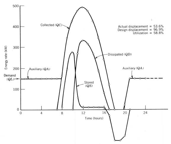
Figure 14.8  Results from program SIMPLESYS for the example case.

 

Starting soon after 4 PM, the rate of energy being supplied by the collector field is less than the demand, and the demand is then supplied by taking energy out of the storage.  By 8 PM, the storage has been depleted and the auxiliary heater takes over the demand until the next morning, when the entire operation is repeated.

 

Table 14.4.  Output for SIMPLESYS Example Case

 

 

The three system performance parameters calculated for this day are also shown.  The output tabulation for this test case indicates that the auxiliary heater supplied 1671 kWh to the 3600 kWh demand.  This leaves 1929 kWh, which was supplied from solar derived energy.  The difference between this and the 3487 kWh collected was dissipated or lost.  The actual displacement then is 1929 kWh divided by 3600 kWh, or a ratio of 54%, and the design displacement is 3487 kWh divided by 3600 kWh or a ratio of 97%.

 

The utilization (of collected energy) does not include the solar supplied energy that is lost from the storage.  For this example day, the net energy supplied to the storage is 120 kWh which is the energy lost from the storage.  The utilization is then 1929 kWh plus 120 kWh, divided by 3487 kWh, or a ratio of 59%.

14.3        Constant Flow System Models

Many solar energy systems operate in a constant flow mode rather than a constant outlet temperature mode as was modeled in SIMPLESYS.  The important difference is that there is no temperature control valve in the collector field outlet line varying the flow through the collectors to maintain a constant outlet temperature.  Instead, the flow through the collector field is constant and the outlet temperature varies with changes in insolation and inlet temperature.

 

Constant flow systems are typically applied to low-temperature applications where auxiliary heating is provided or the temperature at which heat is supplied is not important.  For higher-temperature industrial process heat systems, constant flow systems are in use where the solar collectors provide preheat for boilers, or when the solar boiler is connected in series with a constant-temperature-controlled fossil fueled boiler, which can accept all of the solar-generated steam no mater what the temperature.

 

A constant flow version of SIMPLESYS could be developed using the background developed here.  The collector field model used here would have to be replaced with an iterative routine that would predict the inlet and outlet collector field temperature using a model for collector performance that provides collector outlet temperature as a function of collector inlet temperature and the solar radiation.  It is understood that there are a number of these computer models available.